Burns Snodgrass Navigations Probleme
Burns Snodgrass (1886-1954) war Lecturer für Maschinenbau am Brighton Technical College. Er gründete 1920 eine Rechenschieber Manufaktur "UNIQUE", und stellte eine Reihe spezieller Rechenschieber für Ingenieure her. Die Rechenschieber waren in England und den Kolonien sehr beliebt — sie waren preiswert. Die Firma wurde 1951 umbenannt in "Unique Slide Rule Company Of Brighton Limited"; sie stellte ab 1975 keine Rechenschieber mehr her und wurde in Unique Instruments Ltd. umbenannt. Im Jahr 1994 auf dem Firmenverzeichnis gelöscht (letzter Geschäftsführer: Elaine Snodgrass).
Ich vermute, aus den Anleitungen zu den verschiedenen Sonderausführungen wurde posthum das Buch "Teach Yourself the Slide Rule" (1955) im Verlag The English Universities Press Ltd (heute Hodder Education) verlegt. Als Hinweis verstehe ich, dass es je ein Kapitel zu den bekannten Spartenrechenschiebern gibt:
- Navigational Slide Rule
- Commercial Slide Rule
- Precision Slide Rule
- Electrical Slide Rule
- Dualistic Slide Rule
- Brighton Slide Rule
Außerdem sind offensichtlich einige Absätze im Kapitel "Navigational Problems" bei der Neuerfassung für den Druck "verrutscht"; ich gebe sie aber in der Reihenfolge wie im Buch wieder.
Die Firma Unique stellte auch einen Chemical Slide Rule her, eine Abbildung und eine Anleitung zur Benutzung hat Tina Cordon. Er hat weniger Skalen als meine Rechenschieber für Chemiker von Nestler und Faber-Castell, und scheint sich an das Konzept von William Hyde Wollaston anzulehnen. Er ist gedacht für volumetrische Analysen (Titration).
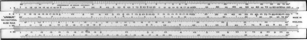
Hier interessiert nur der Navigationsrechenschieber. Der ist aber durch seine Skalenanordnung bemerkenswert: außer den üblichen A/B (x2) und C/D (x) Skalen hat er je eine Sinus- und Tangensskala (S1, S1 und T1, T2) auf dem Körper und der Zunge. Und die sind in Minuten unterteilt. Interessant sind einige der Aufgaben, die durch die besondere Anordnung der Skalen leicht zu lösen sind. Hier ein Auszug: (zur Erklärung der Fachbegriffe)
I gratefully acknowledge the publisher's, Hodder & Stoughton, London, response to my request for permission to use this chapter on my website:
- "We consider your request to use this material as reasonable and fair; therefore you do not need permission from us."
Navigational Problems
The reader will understand that it is not the function of this book to teach the principles of any branch of science or to establish formulae. The book embraces examples dealing with energy, friction, heat, deflection of Beams, strength of shafts, electricity, building, etc., and in no case do we deal with the underlying principles of any of these subjects. We are attempting to show how the slide rule can be employed quickly and easily to cope with the numerous computations which arise. For the principles and formulae involved, the reader must consult the textbooks which are available if he needs such assistance. He will find several such textbooks in the Teach Yourself series.
One of the really fascinating characteristics of the slide rule is the ease with which it deals with some of the problems in trigonometry which are encountered during the navigation of a coasting or sea-going ship, or of an aircraft. There are many proportional problems which arise in connection with aircraft or ships which have no bearing on navigation. For example, the time taken to cover a given distance for a known speed of craft, fuel consumption, con-version from one set of units to another, stowage and loading calculations. Problems of draught and trim and stability.
These problems require no use of trigonometry but can be solved with the aid of the C and D scales or with the use of the other scales we have already examined. We shall not include any examples of these types of problems, but proceed to examine some of those which demand trigonometrical treatment.
We shall, for the remainder of this section, use the Navigational rule which, in the 10″ size, gives a satisfactory degree of accuracy for most problems. We would, however, mention that, if used, the 10/20 Precision rule or the Precision scales of the 10″ Dualistic rule will invariably give a higher degree of accuracy. The disadvantages of using these rules lies in the fact that the values of sines and tangents must be taken from tables, since the trigonometrical scales are not included in the scale equipment of these two rules.
It will be noticed that more space is devoted to navigational problems in Section 7 than to any other single subject. This is because the Navigational rule which is the subject of this section, was designed to deal with the trigonometrical work involved in navigation and we felt that some additional exercises should be given. This rule was introduced in the early days of World War II for the benefit of air navigators, and it will be seen that the data given on the back of the rule, and the scales on the edges, are more concerned with air navigation than with ship navigation, but the problems met with in the two branches of navigation are generally similar and sometimes identical and the Navigational slide rule can be just as easily used for problems arising in ship navigation. The notes on air navigation were contributed by an experienced air navigator.
The slide rule may often be used instead of the traverse table.
- Example: An 8½′ pole standing vertically on a horizontal plane casts a shadow 18′ 3″ long. Calculate the altitude of the sun at the time of observation.
- Over 85D set 1825C.
- Move X to 1C.
- Under X read 25T1.
- Answer: altitude is 25°.
- Example: A ship steering 10° S. of E. observes a light bearing 40° N. of E. After steaming 8 miles the light bears 15° E. of N. Calculate the distances to the light at the two observations.
- 1st angle from the bow =50°,
- 2nt angle from the bow =85°
- Over 35S2 set 8A.
- Over 50S2 read 107A.
- Over 85S2 read 139A.
- Distances 13.9 miles and 10.7 miles.
 Die trigonometrische Ableitung der Formel zu diesem Beispiel wird unter Versegelungspeilung hergeleitet.
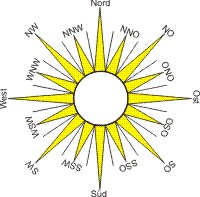
Die Richtungsangaben der Beispiele und Aufgaben folgen denen der Kompassrose. Die Winkel (90°) zwischen den Kardinalrichtungen (N, O, S, W) werden halbiert (NO, SO, SW, NW), und die Winkel zwischen diesen ein weiteres Mal (NNO, ONO, OSO, SSO, usw.). Dazwischen (11¼°) liegen die (Steuer-)Striche: Nord zu NNO, O zu NNO, usw.
Die in den Beispielen angegebenen Peilungsrichtungen beziehen sich auf die Kielrichtung des Schiffes, die "Deckspeilung".
- Problem 29. A ship sailing due N. sights two gas buoys bearing 020° and 035°. After sailing 8 miles the two marks were in line dead abeam. Calculate the distance between the two buoys.
- Example: From a vessel steaming on a straight course a lighthouse was observed 38° forward from the beam. The light was observed to be exactly abeam after the ship had steamed a further 8.3 miles. Calculate the distance at which the light was passed abeam.
- Over 8.3D set 38T2.
- Under 1C read 106D.
- Answer: l0.6 miles.
- Example: From a vessel steaming on a straight course a lighthouse was observed 38° forward from the beam. The light was observed to be exactly abeam after the ship had steamed a further 8.3 miles. Calculate the distance at which the light was passed abeam.
- Problem 30. Find the answer to the foregoing example if the angle forward of the beam had been (a) 58°; (b) 45°.
The Haversine Formula is sometimes useful in dealing with problems which involve the solution of triangles, given the three sides.
- (Note. — Versine A = 1 - cos A
- Haversine A = Hav A = ½ · (1 - cos A).)
- Hav. A = [(s - b) · (s - c)] ⁄ b · c.
- Hav. B = [(s - a) · (s - c)] ⁄ a · c.
- Hav. C = [(s - a) · (s - b)] ⁄ a · b.
- Problem 31. If a = 7, b = 5, c = 4, find A, B and C.
Die Einführung des Sinus versus erscheint etwas unvermittelt: es gibt keine Anwendung des Cosinussatzes oder des Seitencosinussatzes in den Beispielen.
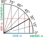
In der Skizze sind der Versin und der Coversin eingezeichnet. Sie wurden in die Astronomie eingeführt, als man mit Logarithmen rechnete, denn sie enthalten nur Produkte von Summen einfach zu berechnender Größen. In den Tafeln war der Logarithmus der beiden Funktionen angegeben.
Zur Ableitung der angegebenen Formeln geht man vom Cosinussatzes in der Form a2 = b2 + c2 - 2 · b · c · cos α aus. Man ergänzt mit + 2 · b · c - 2 · b · c = 0 und faßt den Ausdruck zusammen zu
a2 = (b + c)2 - 2 · b · c · (1 - cos α). Dieser Ausdruck wird aufgelöst nach (1 - cos α):
(Zur Umformung des Zählers siehe Ableitung des Cotangenssatzes!) Jetzt braucht man nur noch 2 · (a + b + c) einzusetzen, und schon hat man den Ausdruck für den Sinus versus.
Navigational Units and Formulae
- Length of nautical mile at Equator, 6046 ft.
- Length of nautical mile at Poles, 6108 ft.
- Standard nautical mile (used in practice), 6080 ft.
- 1 knot = 1 nautical mile per hour.
- 1 cable = 600 feet.
-
dep. = D. long. x cos mid. lat. = D. lat. x tan course. = dist. x sin course. D. lat. = dist. x cos course. = dep. x cot course. tan course = dep. ⁄ D. lat. D. long. dep. x sec mid. lat.
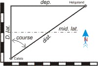 Die hier angegebenen Formeln beziehen sich auf die Berechnung nach der Methode der mittleren Breite. Zur Erklärung der Begriffe siehe nebenstehende Skizze.
Hier wird auch die Winkelfunktion Secans "sec" verwendet. Der ist definiert als Hypotenuse ⁄ Gegenkathete, oder als Kehrwert der Sinusfunktion (sec α = sin-1 α).
In Tabellenwerken für die Navigation werden auch die Werte des Secans und des Cosecans neben denen für Sinus, Cosinus, Tangens und Cotangens angegeben. (z. B. im "The American Practical Navigator" von Nathaniel Bowditch — auch in der Ausgabe von 2002! "csc" ist der Cosecans.)
- Example: A ship steering a course S. 28° E. is making a speed of 14 knots. Calculate the D. lat. and dep. over a 3-hour run.
- D. lat. = dist. x cos course.
- Set 42A over 90S2
- Over 28S2 read 197A.
- Over 62S2 (compl. course) read 370A.
- Answer: D. lat. 37′ departure 19.7′ E.
- Problem 32. Given lat. 24° N. and departure 32 miles, find D. long.
- Example: A ship steamed on a course of 055° for 4 hours at a speed of 18 knots. Calculate the departure and D. lat.
- Distance is 72 miles.
- Course angle is 55°.
- use dep. = dist. x sin course
- D. lat. = dist. x cos course
- Set 90S2 under 72A.
- Over 55S2 read 59A.
- Over 35S2 read 41.2A.
- Answer: Departure 59 miles E.; D. lat. 41.2′ N.
- Example: A ship steamed on a course of 055° for 4 hours at a speed of 18 knots. Calculate the departure and D. lat.
- Problem 33. A ship steamed on a course of 300° for a distance of 400 miles. Calculate D. lat. and departure.
- Example: Calculate the distance from a light known to be 110′ above sea-level at the time when the light first appears above the horizon. Height of observer′s eye 50′.
- Use the formula on [page 106: √H × .98] for distance of sea horizon 1.15 · √H.
- Set 1B under 50A.
- Under 115C read 8125D.
- Set 1B under 110A.
- Under 115C read 1207D.
- Distance 8.125 + 12.07 = 20.195 miles.
- Problem 34. The Spurn Light is 120 ft. high. At what distances will it be just visible to an observer on the bridge of a ship, at height of eye of (i) 20ft.; (ii) 40ft.; (iii) 60ft.?
Wind and Drift Problems
To find the course to steer and ground speed along given track.
Using scales S2 and A. Under the airspeed set the angle on the bow or quarter of the track that the wind is blowing. Under the wind speed read the drift angle. The drift angle, added or subtracted to the track, will give the course to steer.
To find the ground speed: if the wind is a head wind, subtract the drift angle from the wind angle on the bow; if a tail wind, add the drift angle to the wind angle on the quarter. Above the resulting angle read the ground speed.
- Example: Airspeed 126 m.p.h. Track 040° T. Wind velocity 20 m.p.h. from 090° T. (50° on the bow).
- To 126A set 50S2.
- Under 20A read 7S2.
- Over 43S2 (50° - 7°) read 112A.
- Result: Course to steer 043° T.; ground speed 112 m.p.h.
- Example: Airspeed 97 knots. Track 352° T. Wind velocity 15 knots from 110° T (62° on the starbd. quarter).
- To 97A set 62S2.
- Under 15A read 8S2 (drift).
- Over 70S2 (62° + 8°) read 103S2.
- Result: Course to steer 360° T.; ground speed 103 knots.
- Note that when the drift is less than 1 degree, the ground speed should be found by adding or subtracting the wind speed and the airspeed.
Hier wird der Sinussatz zur Berechnung des scheifwinkligen Dreiecks angewandt. Bei der Berechnung zeigen sich die Vorzüge der Winkelfunktionsskalen auf der Zunge. Man löst die Aufgabe mit einer Einstellung durch Verschieben des Läufers.
To find the wind velocity, knowing the track and ground speed, course and airspeed.
On scale A mark the airspeed and ground speed with the cursor and a light pencil mark. Adjust the slide until the number of degrees read between the airspeed and the ground speed markings equals the drift angle, i.e. the difference between the course and the track. Above the drift angle on scale S2 read the wind speed on scale A. Under the airspeed read the wind direction as an angle on the bow or quarter of the track, or under the ground speed as an angle on the bow or quarter of the course. Note that if the G/S is less than the A/S, the angle is on the bow, and if the A/S is less than the G/S, an angle on the quarter.
- Example: Course 137° T. Airspeed 150 m.p.h. Track 142° T. Ground speed 130 m.p.h.
- Mark the scale A at 130 and 150. Adjust the slide until a difference of reading of 5 degrees on scale S2 is obtained between the above markings. In this example 29° and 34° will be found to correspond. On scale A above 5° read 23.4 m.p.h. (wind speed). The wind direction is 34° on the bow of the track and is therefore 108° T. as the drift is to starboard.
To find the wind speed and ground speed, knowing the course and airspeed, drift angle and wind direction.
This method is particularly useful when a flight is being made over the sea and it is desired to know the ground speed. In such cases the drift angle can nearly always be found by a drift sight or back-bearings of an object dropped from the aircraft, but it is not such a simple matter to determine the ground speed. It is a known fact, in a steadily moving air mass, the difference between the wind direction at the surface and the wind direction at a reasonable height remains nearly constant with the changes of surface wind direction.
This difference can be ascertained at the departure point from meteorological information available and applied to the direction of the surface wind obtained during the flight by bearings of the wind lanes on the sea surface. It has also been found that in practice a reasonably accurate forecast of the direction of the upper winds can be given by a meteorologist, whereas difficulty is sometimes experienced in to recasting the speed. The wind direction can also be ascertained by noting the direction of movement of cloud shadows on the surface.
With these various sources at the navigator′s disposal little difficulty is usually encountered in finding the wind direction.
- Example: Airspeed 110 knots. Course 136° T. Track 142° T. Drift 6° to starbd. Wind direction 348° T.
- The difference between the track and wind direction is 206°. The wind angle is therefore 26° on the quarter, a tail wind. Therefore 26° added to 6° (the drift) will give the angle to use to find the ground speed.
- To 110A set 26S2.
- Over 6S2 read 26.2 (wind speed).
- Over 32S2 read 133 (ground speed).
- Result: Wind speed 26.2 knots; ground speed 133 knots.
To find the new track and ground speed after an alteration of course.
This method is not mathematically correct, but is sufficiently accurate when it is desired to know the track and ground speed immediately after an alteration of course. In practice, drift should be checked by observation as soon as possible after any alteration of course, so it should never be really necessary to calculate the D.R. track.
- Example: Before alteration of course the track was 045° T. Windvelocity 20 m.p.h. from 095° T. True airspeed 140 m.p.h. Drift 6¼°. Course steered 051° T. Course is altered to 120°. The wind is now 25° on the port bow of the aircraft, previously it was 44° on the starbd. bow.
- To 6.25A set 44S2.
- Over 25S2 read 3.8A.
- Result: The new drift is 3° 48′, and the new track is 124° to the nearest degree.
- To find the new ground speed:
- To 20A set 3° 48′ S2 (wind speed).
- Move X to 140A.
- If the angle under the cursor is not an even degree or half degree, adjust the slide accordingly, to bring the nearest half or whole degree under the cursor. Then move the cursor 3° 48′ to the left (as the wind is ahead) and read on scale A the new ground speed. 122½ m.p.h.
If course is being altered frequently, as it would be if a search of some kind were being carried out, it would be far easier and decidedly more accurate to keep a plot of air Courses on the chart. When it is desired to know the D.R. position, the total windage affecting the aircraft during the search can be applied to the air position. This can most effectively be accomplished by plotting a wind scale, subdivided into intervals of, say five minutes. The distance that the aircraft has been blown downwind can then be conveniently stepped off with dividers from the air position.
Thus if the air courses flown have totalled 55 minutes from the last fix, then 55 minutes of wind is used. The wind scale is, of course, constructed to the same scale as the distance scale of the chart or map.
It should always be borne in mind that the errors of D.R. navigation are accumulative; therefore the more observations of drift, ground speed or position that can be made, the more accurate will be the final result. It will be seen in all these problems that the drift angle is always subtracted from the wind angle to the track for head in remembering this, for it will always be readily seen when using the slide rule, for a head wind will always reduce the ground speed, and a tail wind will increase it.
Interception Problems
In theory, the most accurate method of determining the course to steer to intercept a moving surface-vessel is by plotting, and for examination purposes this is the safest method to adopt. In practice, however, this very seldom works out, because changes of wind or weather en route often necessitate an alteration of course, and consequently the time and labour spent in solving the original problem is wasted. Again, the problem often arises: When the ground speed during the flight is not what it was estimated to be, how much has course to be altered? Theoretically, a new interception problem should be worked out, but this is a rather lengthy procedure. The following method, using the slide rule, gives a simple solution to this type of problem.
- Example: Bearing and distance of ship 012° 282′. Ship′s course and speed 125° 17 knots. Airspeed 120 knots. Wind velocity 22 knots, from 247°.
- Find the angular difference between the relative bearing and the ship′s course, i.e. 125° - 12° = 113° or 67° on the "quarter" of the relative bearing. Estimate the ground speed of the aircraft. This can be done quite roughly, as a few knots either side of the correct ground speed is negligible. Ground speed is therefore estimated to be 125 knots.
- Under 125A (G/S) set 67S2.
- Traverse slide.
- Under 17A (ship′s speed) read 7° 11′S2.
- This will give the angle the track out makes with the relative bearing. The track is therefore 019° T. Find now the angular difference between the wind direction and the track. 019° + 180° = 199° - 247° = 48° on the quarter.
- Under 120A set 48S2.
- Under 22A read 7° 50′S2.
- Over 55° 50′S2 read 133½A.
- As the wind is a tail wind, 7° 50′ and 48° are added, and the true ground speed out is 133½ knots. If the first part of the problem is re-checked, using the correct G/S of 133½ knots, it will be seen that the angle between the relative bearing and the track is still approximately 7°.
- The drift has been found to be 7° 50′ starboard. The Course to steer is therefore 011°.
- Find the angular difference between the relative bearing and the ship′s course, i.e. 125° - 12° = 113° or 67° on the "quarter" of the relative bearing. Estimate the ground speed of the aircraft. This can be done quite roughly, as a few knots either side of the correct ground speed is negligible. Ground speed is therefore estimated to be 125 knots.
If, after the course has been set, an alteration in the estimated ground speed is discovered, the amount which course has to be altered (to maintain the relative bearing of approach) can be found by carrying out the procedure adopted in the first part of this example, using the new ground speed, and thus finding the new track to intercept. This track can then be maintained by drift observations and slight alterations to course. During the latter stages of the fiight, if large changes of drift or ground speed are found, a new relative bearing should be measured between the calculated D.R. positions of the ship and the aircraft, at the same instant of time. If this is done for a few minutes ahead, and a change of relative bearing is discovered, the new course to steer can be determined by using the new angle between the new relative bearing and the ship′s course.
The estimated time of interception should be calculated by measuring the distance along the track, and applying the measured ground speed. If the speed of closing is used along the line of relative bearing, same difficulty will been countered in the calculation of a new E.T.I. when it is found that the G/S is not what it was estimated to be.
Die Trigonometrie und der Rechenweg dieser Aufgabe ist für Schiffe unter Treffpunktproblem erläutert. Mit Sinusskalen auf Körper und Zunge — wie beim UNIQUE NAVIGATOR — ist die Berechnung mit weniger Schritten zu bewältigen.
The Calculation of True Track and Distance
The true track and distance by the middle latitude formula.
- Formula:
- dep. = D. long. · cos mid. lat.
- tan tr. = dep. ⁄ D. lat.
- dist. = dep. · cosec tr.
- D. lat. · sec tr.
To find the rhumb line and track from Calais to Heligoland.
| Calais | lat. | 50° 58′ N. | long. | 1° 51′ E. |
| Heligoland | lat. | 54° 11′ N. | long. | 7° 53′ N. |
| D. lat. | 3° 13′ N. | D. long. | 6° 02′ | |
| 193′ | 362′ | |||
| mid. lat. | 52° 34.5′ | |||
To find the departure.
- Set 362B to 90S1
- Under 37° 25½81 (comp. of mid. lat.).
- Read 220B.
- Departure 220′
To find the true track.
Rule: Always set the larger value af D. lat. and dep. on scale C, and the smaller value an scale D.
- Over 193D set 220C.
- Set X to 10C.
- Under X read 41° 15′ in T1.
As the dep. is greater than the D. lat. the track is obviously greater than 45°. Therefore the complement of the angle 41° 15′ is used. The track is always named the same as the D. lat. and the D. long.
True track = N. 48° 45′ E. or 049° T. to the nearest half degree.
To find the rhumb line distance.
- Set X to 48° 45′ S1 and move 220B to X.
- Under 90 S1 read 293B.
- Rhumb line distance 293 nautical miles.
To find the rhumb line track and distance from Calais to Gibraltar.
| Calais | lat. | 50° 58′ N. | long. | 1° 51′ E. |
| Gibraltar | lat. | 36° 04′ N. | long. | 5° 26′ W. |
| D. lat. | 14° 54′ S. | D. long. | 7° 17′ W. | |
| 894′ | 437′ | |||
| mid. lat. | 43° 31′ | |||
To find the departure.
- To 90S1 set 437B.
- Under 46° 29′S1 read 317B.
- Departure 317′.
To find the true track.
- Over 317D set 894C.
- Set X to 10C.
- Under X read 19° 30′T1.
- True track S. 19½° W. or 199½° true.
To find the rhumb line distance.
- Set X to 19° 30′S1.
- Set 317B to X.
- Under 90S1 read 951B.
- Rhumb line distance 951 nautical miles.
Distances of over 200 miles should always be calculated in preference to measuring the distance by dividers on the map or chart. Again, it is always easier and more accurate to calculate the track and distance between places which are not on the same map or chart sheet. A little practice with the slide rule will enable this problem to be solved more accurately, and in a shorter time than it would be if traverse tables were employed.
The great circle track and distance, etc.
In air navigation, the great circle track has other uses than the saving in distance during a long flight. It can be used to avoid ranges of high mountains or prohibited areas without increasing the distance flown, and in flights, when it is desired to bring the track of the aircraft within visibility distance of some landmark, to assist navigation, when by flying the rhumb line track the landmark would have been missed altogether. It is, of course, not always possible to utilise the great circle track in this manner, but these advantagcs should not be forgotten when planning a flight of even moderate distance.
To calculate the problems involved, by spherical trigonometry, is a very tedious procedure. When, in order to shorten the work, short tables are employed, an added disadvantage is encountered, namely the necessity of having to choose two points near the departure point and destination to obtain angles to fit the tables.
By using the slide rule all these difficulties are overcome, for the solution is both rapid and accurate, and the actual positions of the chosen places can be used.
To calculate the great circle distance.
Formula:
- tan lat. A × tan lat. B + cos D. long.
- (If lat, A and B are in the same hemisphere.)
- tan lat. A × tan lat. B - cos D. long.
- (If lats. A and B are in different hemispheres.)
- The result is called C.
- C × cos lat. A × cos lat. B = cos distance.
N.B. - The rules regarding the plus and minus to D. long. are reversed if the D. long. exceeds 90°.
Example: Position A, lat. 38° 45′ N., long. 9° 30′ W. Position B, lat. 40° 25′ N., long. 73° 15′ W. Difference of longitude is 63° 45′ W.
- Over 38° 45′T1 set 45T2.
- Under 40° 25′ T2 read 683D.
- i.e. tan lat. A × tan lat. B = .683.
- Under 26° 15′S1 (comp. 63° 45′).
- Read 442A i.e. cos D. long. = .442.
- .683 + .442 = 1.125 (as A and Bare in the same hemisphere).
- Under 51° 15′S1 set 90S2 (comp. lat. A).
- Move X to 49° 35′S2 (comp. lat. B).
- Set 1B to X.
- Read 48° 03′S1 over 1.125B.
The angle 48° 03′ is read as a complementary angle to that indicated on scale S1 as the answer is the cosine of the distance.
Great circle distance 48° 03′ or 2883 nautical miles.
In the latter process the formula is 1.125 × cos lat. A × cos lat. B = cos distance.
Note that the scales S1 and S2 are sine scales, and to use these scales for cosines the complementary angles must be used. After becoming acquainted with the use of the trigonometrical scales, the beginner will be able to select the complements of angles quite easily from the sine scale by counting the degrees from the right-hand index, or from an easily recognised complement, e.g. 60°, 45° or 30°.
The initial track.
Formula:
- sec lat. A × sin lat. B × cosec distance = A (opposite name to lat. A).
- tan lat. A × cot dist. = B ( same name as lat. B).
The algebraic sum of A and B is the cosine of the initial track. Lat. A 38° 45′ N. Lat. B 40° 25′ N. Distance 48° 03′.
To find A.
- Under 51° 15′S1 (comp. 38° 45′) set 40° 25′S2.
- Move X to 48° 03′S2.
- 100B to X.
- Under 90S1 read 112B.
To find B.
- Over 38° 4S′T1 set 45T2.
- Under 41° 57′T2 (comp. dist.) read 721D.
- 1.12.- .721 = .399 (see rules above)
- (A is South, B is North).
.399 is the cosine of 66° 30′. This is read from the scales A and S1 by setting the Cursor over the required figures. Initial track N. 66½° W. or 293½° T.
To find the latitude of the vertex.
Formula:
- sin init. tr. × cos lat. dep. = cos lat. vertex.
- init. course 66° 30′. lat. dep. 38° 45′ N.
- Set 90S2 under 66° 30′S1.
- Over 51° 15′S2 read 44° 20′S1 (as a cosine).
- Lat. of vertex: 44° 20′ N.
To find the longitude of the vertex.
Formula:
- cosec lat. dep. × cot init. tr. = tan difference of longitude between point of departure and longitude of vertex.
- lat. of dep. 38° 45′ N. Init. tr. 66° 30′.
- Under 38° 45′S1 set 100B.
- Under 1A read 16B.
- Over 16D set 1C.
- Under 23° 30′T2 (comp. 66° 30&prime) read 34° 50′T1.
The longitude of the vertex will be 34° 50′ W. of the point of departure, and will therefore be in long. 44° 20′ W.
To find the latitudes in which the great circle track will cut given meridians.
Formula:
- tan lat. = tan lat. vertex × cos D. long. between the longitude of the vertex and the given meridian.
- Meridian 19° 30′ W. Lat. vertex 44° 20′ N. D.long. is 24° 50′.
- From scales A and S1 find cos D. long. 24° 50′ equals .907.
- Over 907D set 45T2.
- Under 44° 20′T2 read 41° 33′T1.
- Lat. of tr. in meridian 19° 30′ W. = 41° 33′ N.
To find the track in any latitude.
Formula:
- sin tr. = sec lat. × cos lat. vertex. Chosen lat. 40°.
- Lat. of vertex 44° 20′ N.
- Under 90S1 set 50S2 (comp. of 40°).
- Over 45° 40′S2 (comp. 44° 20′) read 69S1.
- Lat. of vertex 44° 20′ N.
- Tr. in lat. 40° N. is N. 69° W. or 291° T.
For calculation of a D.R. or air position.
Formula:
- dep. = dist. × sin tr.
- D. lat. = dist. × cos tr.
- D. long. = dep. × sec mid. lat.
To find the D.R. position after a run of 3 hours along a track of 242° T. at a G/S of 138 knots, from a position lat. 50° 30′ N., long. 9° 20′ W.
242° T. is a bearing of S. 62° W. 3 hours at 138 knots represents a run of 414 nautical miles.
To find the departure.
- Under 414A set 90S2.
- Over 62S2 read 365A.
- Departure 365′.
To find the difference of latitude.
- Under 414A set 90S2.
- Over 28S2 (comp. of 62°) read 194.5A.
- D. Lat. 194′.5 or 3° 14′.5 S. (named S. because the tr. is S.).
(Note that both these problems can be solved together with one setting of the slide by moving the cursor from the course on scale S2 to the complement of the course, thus multiplying by the sine in the first case, and by the cosine in the second.)
To find the difference of longitude.
The middle latitude is obtained by applying half the D. Lat. found to the latitude of the departure position. Thus the Mid. Lat. is 48° 53′.
- Under 365A set 41° 07′S2 (comp. mid. lat.).
- Over 90S2 read 556A.
- D. Long. 556′ or 9° 16′ W. (named W. because the tr. is W.). The D.R. position is therefore lat. 47° 15′.5 N. Long. 18° 36′ W.
This process of calculating the D.R. position is very useful when changing from one chart to another, especially if the charts are of a different scale, or when greatcr accuracy is required than can be obtained by measuring a long distance run an a chart with a varying scale of latitude.
If it is desired, the course and airspeed of the aircraft can be used to calculate an air position. When the geographical position is required the wind velocity is applied as an additional track and distance. This "track" will represent the direction of the wind (downwind), and the distance will be the distance the aircraft has been blown downwind, during the time of flight at the given wind speed.
The use of pre-computed lines of position.
When a long flight is being carried out above layers of clouds, or over the high seas, and astronomical navigation is being employed, it is very convenient sometimes to compute the calculated altitude before the observed altitude is taken. This saves time if course has to be altered as a result of the observation made, and it enables most of the work to be done when the navigator is fresh and not flurried.
Knowledge of the estimated track and ground speed of the aircraft will enable its D.R. position to be plotted for every hour or half-hour of the flight. Using these positions and the G.M.T. of each E.T.A., calculate the individual altitudes of the chosen heavenly body.
When in flight, and the time approaches for the first observation, take the series of sights as near as possible to the G.M.T. which was used for the calculated altitudes. The pre-computed altitude can be corrected for any slight difference of time by the following formula:
- Correction = cos lat. × sin az. × ¼ · (diff. in secs.).
- Example: Pre-calculated altitude 36° 47′, azimuth S. 47° W. G.M.T. 15 hrs. 06 mins. 00 secs. D.R. lat. 48° N. G.M.T. of observation 15 hrs. 07 mins. 06 secs. Obs. alt. 36° 23′. Difference 66 secs.
- Under 42S1 set 90S2.
- Move X to 47S2.
- Set 90S2 to X.
- Move X to 66B.
- Set 40B to X.
- Over 100B read 8.1A.
The correction to pre-computed altitude is 8.1 minutes. As the hour angle is westerly, the body is decreasing in altitude. The correction is therefore subtracted and the calculated altitude to use is 36° 39′ and the intercept will be 16 miles away.
The fix by horizontal angles.
The horizontal angle between two points results in a circle of position, the radius of which is obtained by the formula:
- .5 · d ⁄ sin θ
where d = the distance between the points and θ = the horizontal angle.
The intersection of two circles of position will give the position of the observer.
Although this problem can be solved by using a station pointer or a protracter, these instruments are not always convenient to use on all charts. By using the slide rule to solve the problem of finding the radii of the circles of position, and determining the centres of these circles by construction, an accurate and simple method is always at hand.
- Example: A and B are two objects 6 miles apart, and C a third object 8.6 miles from B. The horizontal angle between A and B is 68° and between B and C 56°. Required the radii of the two circles of position.
- Under 68S1 set 6D.
- Under 5A read 3.23B.
- Under 56S1 set 8.6B.
- Under 5A read 5.19B.
- The respective radii are 3.23 and 5.19 miles respectively. Arcs made, using each pair of objects, and the radius applicable will determine the centres of the required circles of position, and the intersection of arcs from these centres will give the position of the observer.
Although a fix by this method is not very practicable when airborne, it is invaluable when a survey of an advanced landing-ground or anchorage is being carried out.
Hier wird ein Rechenbeispiel für die Positionsbestimmung durch zwei Horizontalwinkel angegeben.
To find conversion angle.
Formula:
- ½ · D. long. × sin mid. lat. = conversion angle.
- D. long. 6° 40′. Mid. lat. 62°.
- Under 6° 40′S1 set 90S2.
- Move X to 62S2.
- Set 90S2 to X.
- Over 5B read 2° 56′S1.
- Conversion angle = 2° 56′.
Numerous rules have been proposed which are purported to aid the navigator in remembering how conversion angle should be applied. If it is remembered that no matter whether the latitude is North or South, or whether the bearing is from a shore station or from the aircraft, the conversion angle correction is always applied towards the Equator, no difficulty will be encountered.
Radius of action.
The problem of finding the radius of action of an aircraft along a given track for a known endurance is a very simple matter if the slide rule is always employed.
Formula:
- [(G/S out × G/S home) ⁄ (G/S out + G/S home)] × fuel hours = radius of action.
Example: Airspeed 230 m.p.h. Track out 040° T. Wind velocity 20 m.p.h. from 102° T. Fuel hours 35.
- Wind is 62° on the bow.
- Set X to 230A. 62S2 to X. X to 20A.
- Under X in S2 read 4½° (drift).
- Over 57½ S2 read 220A = G/S out (against wind).
- Over 66½ S2 read 239A = G/S home (with wind)
- 220 + 239 = 459.
- To 220 set 1C. X to 239C. 459C to X.
- Read in D under 35C radius of action, 4010 nautical miles.
- The time to turn is found from the time required to fly the 4010 miles at the outward G/S.
To find the error in track from a position line parallel to the D.R. track.
When navigating by astronomical observations, every advantage should be taken to observe heavenly bodies abeam of the aircraft, as the resulting position Iines will give a good indication of the true track of the plane.
If no terrestrial observations have been possible since the departure, it will be desired to know the error in the course being steered. This can be easily found as follows.
Example: After flying 186 miles an observer obtained a position line placing the aircraft 38 miles to Starboard of the D.R. track. Find the error in the track.
- Over 380 set 186C.
- Under 1C read 11½T1.
- The Track error is 11½°.
This method can also be employed when navigating over land, or when D/F W/T bearings are being used. It can also be used to give the alteration of course required to reach a certain destination, when of course the distance of the aircraft from the destination should be used instead of the distance run since departure.
It might be noted here that when sights are being taken to make a running fix, a sight of a heavenly body on the beam should invariably be taken first, as it will not then be necessary to transfer this position line for the "run" between it and the next observation. It will be found sufficiently accurate in practice to extend the position line until it cuts the line resulting from the second sight, thus giving a fix and saving one the labour of transferring the observation for the time interval between sights.
Correction of refraction.
Altitudes above 8°. Multiply the cotangent of the altitude by .96.
Altitude 36°, required the correction for refraction.
- Over 36T1 set 96C.
- Over 1D read 1.3C (to nearest first place of decimals).
- Correction is 1.3 minutes minus to the apparent altitude.
Correction for dip of the sea horizon.
Example: An observer flying at 840 ft. above sea-level requires the dip correction.
- Set X to 840A.
- Set 10C to X.
- Under 98C read 284D.
- Dip Correction is 28.4 minutes minus to the observed altitude.
To find the distance to the sea horizon.
Formula: √height × 1.15. The resulting distance is given in nautical miles.
Wenn man die Höhe in Metern misst (statt wie Sondgrass in feet), ist der Faktor 1,777.
To find the distance of an object from the angle of depression.
For distances up to ten miles.
Formula:
- .565 · H ⁄ θ = distance in nautical miles = D1.
- H = height of observer in feet above the object.
- θ = angle of depression in minutes.
For distances over ten miles or for greater accuracy.
- Formula: .565 · H ⁄ (θ - .4 · D1) = D2.
- D1 and D2 distances in nautical miles.
D1 should be found, using the first formula, and then when .4 · D1 is obtained the second formula can be used to calculate the final result.
To find D1.
- Over 565D set θ in scale C.
- Under H in scale C read D1 in scale D.
To find D2.
- Over 565D set θ - .4 · D1 in scale C.
- Under H in scale C read D2 in scale D.